P-value of detection: null
False Discoveries across entire molecule (length*p-value): null
Probability of true detection (1.3=90%): 1-pnorm( - null )
NOTE: the numerics of the statistical test in javascript sometimes
differ from R, use with caution.
Also sometimes the page outputs error, just re-enter inputs and try
again.
Other codon analysis filters to correct codons. This will decrease the error rate.
================================
Methods:
To do minor variant detection, estimate whether minor variant counts
in independent columns:
- are due to noise or
- have excess of counts due to the presence of a true minor variant
For illustration, assume noise gives false observations of a minor
variant at a rate of 5%. A minor variant occurs at the rate of 1%. The
simplified problem is to differentiate the 6% of the variant from the
5% of the noise. At first this might seem difficult because the minor
variant level is below the noise level, but we can use statistics from
multiple observations to reliably separate the two cases.
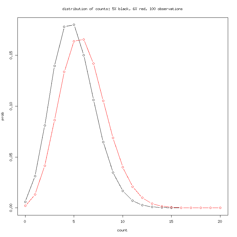
The distributions are over overlapping, almost impossible to
differentiate with 100 observations.
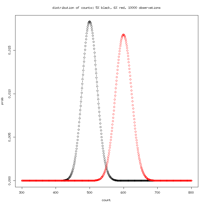
The distributions are distinct with little overlap with 10,000
observations.
The procedure is to sequence and then count how many minor bases there
are out of the total. You can then compare this to a "null control"
run in which there is no minor variant and any minor observation is
due to noise. We use the fisher exact test to test these two
proportions, but other tests can be used.
The code computes significance at observation of the average number of
counts. The false negative rate is therefore 50% because half the
time, you observe less than the average and lose significance of the
detection. In order to decrease the false negative rate, we move left
on the binomal distribtuion and ensure that even with these reduced
counts, the test will be significant. For example if we move -1.3
standard deviations smaller, we decrease the false negative rate to
10% : 1-pnorm(-1.3)=90%.
Here is the R code:
# inputs
N=4000 # num reads
A=0.01 # Minor abundance
E=0.02 # read error rate CCS=1%
sigM = 1.3 # (1-prob(detect). How many fewer counts to threshold to increase from 50% FNR. 1-pnorm(-1.3)=0.90319995
# caclulate expected observed counts
TP=N*A*(1-E)
FN=N*A*E/4
TN=N*(1-A)*(1-E)
FP=N*(1-A)*(E/4)
# tail sampling for FNR
p = A*(1-E) + (1-A)*(E/4) # the factor to N for (TP+FP)
sampSD = sqrt(N*p*(1-p)) # binomal sampling variance
# test expected counts minus sampling variance is signficantly different from random noise
m = cbind (c( (TP+FP) - sigM*sampSD, N), c( (E/4)*N,N))
mmm=fisher.test(m)
mmm$p.value
[1] 0.0006068087
 The distributions are over overlapping, almost impossible to
differentiate with 100 observations.
The distributions are over overlapping, almost impossible to
differentiate with 100 observations.
 The distributions are distinct with little overlap with 10,000
observations.
The procedure is to sequence and then count how many minor bases there
are out of the total. You can then compare this to a "null control"
run in which there is no minor variant and any minor observation is
due to noise. We use the fisher exact test to test these two
proportions, but other tests can be used.
The code computes significance at observation of the average number of
counts. The false negative rate is therefore 50% because half the
time, you observe less than the average and lose significance of the
detection. In order to decrease the false negative rate, we move left
on the binomal distribtuion and ensure that even with these reduced
counts, the test will be significant. For example if we move -1.3
standard deviations smaller, we decrease the false negative rate to
10% : 1-pnorm(-1.3)=90%.
Here is the R code:
# inputs
N=4000 # num reads
A=0.01 # Minor abundance
E=0.02 # read error rate CCS=1%
sigM = 1.3 # (1-prob(detect). How many fewer counts to threshold to increase from 50% FNR. 1-pnorm(-1.3)=0.90319995
# caclulate expected observed counts
TP=N*A*(1-E)
FN=N*A*E/4
TN=N*(1-A)*(1-E)
FP=N*(1-A)*(E/4)
# tail sampling for FNR
p = A*(1-E) + (1-A)*(E/4) # the factor to N for (TP+FP)
sampSD = sqrt(N*p*(1-p)) # binomal sampling variance
# test expected counts minus sampling variance is signficantly different from random noise
m = cbind (c( (TP+FP) - sigM*sampSD, N), c( (E/4)*N,N))
mmm=fisher.test(m)
mmm$p.value
[1] 0.0006068087
The distributions are distinct with little overlap with 10,000
observations.
The procedure is to sequence and then count how many minor bases there
are out of the total. You can then compare this to a "null control"
run in which there is no minor variant and any minor observation is
due to noise. We use the fisher exact test to test these two
proportions, but other tests can be used.
The code computes significance at observation of the average number of
counts. The false negative rate is therefore 50% because half the
time, you observe less than the average and lose significance of the
detection. In order to decrease the false negative rate, we move left
on the binomal distribtuion and ensure that even with these reduced
counts, the test will be significant. For example if we move -1.3
standard deviations smaller, we decrease the false negative rate to
10% : 1-pnorm(-1.3)=90%.
Here is the R code:
# inputs
N=4000 # num reads
A=0.01 # Minor abundance
E=0.02 # read error rate CCS=1%
sigM = 1.3 # (1-prob(detect). How many fewer counts to threshold to increase from 50% FNR. 1-pnorm(-1.3)=0.90319995
# caclulate expected observed counts
TP=N*A*(1-E)
FN=N*A*E/4
TN=N*(1-A)*(1-E)
FP=N*(1-A)*(E/4)
# tail sampling for FNR
p = A*(1-E) + (1-A)*(E/4) # the factor to N for (TP+FP)
sampSD = sqrt(N*p*(1-p)) # binomal sampling variance
# test expected counts minus sampling variance is signficantly different from random noise
m = cbind (c( (TP+FP) - sigM*sampSD, N), c( (E/4)*N,N))
mmm=fisher.test(m)
mmm$p.value
[1] 0.0006068087