goal: collect together results for bcr-abl paper
================================
Summary:
I give below some results for the bcr-abl paper.
- reduced and clinical merged data table, reduced data table, combined data table
- reproducibility of variant positions that are significant in both
replicates.
- number of mutations versus the number of silent mutations
- look at number of variant positions observed versus number of
compounds > 1%
- time evolution plots of variant positions
- interesting compound variants for CSY and EEC
================================
Combined, reduced, merged variant data table:
I have three sets of data tables (.txt which is tab-separated data
tables). All give the same information but have been reduced and
merged in different ways.
1) reduced and merged with clincial: reduced pacbio data merged with UCSF clinical data (hopefully up-to-date)
2) reduced: this is pacbio data but all results reduced and grouped by patient
3) combined: this is all pacbio data in full form
For each set I give list of variants, list of variants > 1%, list of
compound variants > 1%
---- 1) reduced and merged with clincial:
mutationCollapseMergeClinical.txt for each sampleID the list of mutations
significant in both runs with clinical
mutationCollapseMerge1perClinical.txt for each sampleID the list of mutations
significant in both runs and > 1% with clinical
compoundmutationCollapseMerge1perClinical.txt for each sampleID the
list of compound mutations observed at > 1% with clinical
---- 2) reduced:
mutationCollapseMerge.txt for each sampleID the list of mutations
significant in both runs
mutationCollapseMerge1per.txt for each sampleID the list of mutations
significant in both runs and > 1%
compoundmutationCollapseMerge1per.txt for each sampleID the
list of compound mutations observed at > 1%
---- 3) combined:
NEW.bcrabl.variants.tsv.xls
NEW.bcrabl.variants.significantInBoth.tsv.xls
NEW.bcrabl.compoundvariants.tsv.xls
Here is the data table from the paper
bcrabl.tsv
================================
There are so many possibilities for what to include: structural
variation, quality, silent vs total, num vs numCompound, time
evolution, where the variants occur (single and compound). I have many
many results in all the READMEs for this project. TODO: go through all
readmes for information.
================================
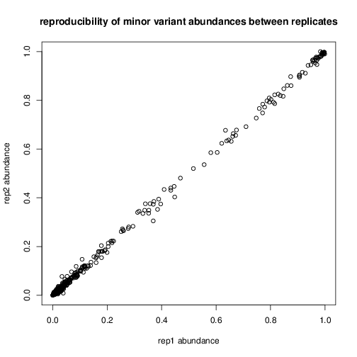
abundance agreements between technical repeats.
 mylm = lm(resultp$frac1 ~ resultp$frac2)
summary(mylm)
Call:
lm(formula = resultp$frac1 ~ resultp$frac2)
Residuals:
Min 1Q Median 3Q Max
-0.043617 -0.001181 -0.000119 0.001133 0.063501
Coefficients:
Estimate Std. Error t value Pr(>|t|)
(Intercept) 0.0001075 0.0001719 0.625 0.532
resultp$frac2 1.0014472 0.0008202 1221.027 <2e-16 ***
---
Signif. codes: 0 ‘***’ 0.001 ‘**’ 0.01 ‘*’ 0.05 ‘.’ 0.1 ‘ ’ 1
Residual standard error: 0.005883 on 1309 degrees of freedom
Multiple R-squared: 0.9991, Adjusted R-squared: 0.9991
F-statistic: 1.491e+06 on 1 and 1309 DF, p-value: < 2.2e-16
RESULT: R-squared of 0.9991, reproducibility is very high. This is
impressive as these were run on different chips at different times and
went through barcoding!
resultp$relerr = 2*abs(resultp$frac1 - resultp$frac2)/(resultp$frac1 + resultp$frac2)
summary(resultp$relerr[2:nrow(resultp)])
Min. 1st Qu. Median Mean 3rd Qu. Max.
0.00000 0.04924 0.12170 0.16310 0.23520 1.27700
RESULT: Median relative error of 12% across entire range.
================================
mylm = lm(resultp$frac1 ~ resultp$frac2)
summary(mylm)
Call:
lm(formula = resultp$frac1 ~ resultp$frac2)
Residuals:
Min 1Q Median 3Q Max
-0.043617 -0.001181 -0.000119 0.001133 0.063501
Coefficients:
Estimate Std. Error t value Pr(>|t|)
(Intercept) 0.0001075 0.0001719 0.625 0.532
resultp$frac2 1.0014472 0.0008202 1221.027 <2e-16 ***
---
Signif. codes: 0 ‘***’ 0.001 ‘**’ 0.01 ‘*’ 0.05 ‘.’ 0.1 ‘ ’ 1
Residual standard error: 0.005883 on 1309 degrees of freedom
Multiple R-squared: 0.9991, Adjusted R-squared: 0.9991
F-statistic: 1.491e+06 on 1 and 1309 DF, p-value: < 2.2e-16
RESULT: R-squared of 0.9991, reproducibility is very high. This is
impressive as these were run on different chips at different times and
went through barcoding!
resultp$relerr = 2*abs(resultp$frac1 - resultp$frac2)/(resultp$frac1 + resultp$frac2)
summary(resultp$relerr[2:nrow(resultp)])
Min. 1st Qu. Median Mean 3rd Qu. Max.
0.00000 0.04924 0.12170 0.16310 0.23520 1.27700
RESULT: Median relative error of 12% across entire range.
================================
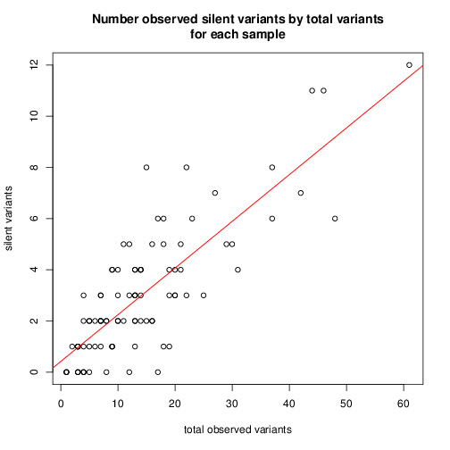
look at the number of mutations verus the number of silent mutations
mylm = lm(silentDat$numSilent ~ silentDat$total)
summary(mylm)
Call:
lm(formula = silentDat$numSilent ~ silentDat$total)
Residuals:
Min 1Q Median 3Q Max
-3.5176 -1.0578 0.0335 0.8984 4.8474
Coefficients:
Estimate Std. Error t value Pr(>|t|)
(Intercept) 0.4155 0.2484 1.672 0.0979 .
silentDat$total 0.1825 0.0136 13.418 <2e-16 ***
---
Signif. codes: 0 ‘***’ 0.001 ‘**’ 0.01 ‘*’ 0.05 ‘.’ 0.1 ‘ ’ 1
Residual standard error: 1.486 on 90 degrees of freedom
Multiple R-squared: 0.6667, Adjusted R-squared: 0.663
F-statistic: 180 on 1 and 90 DF, p-value: < 2.2e-16
About 18% of observed minor variants are silent with significance.
 ================================
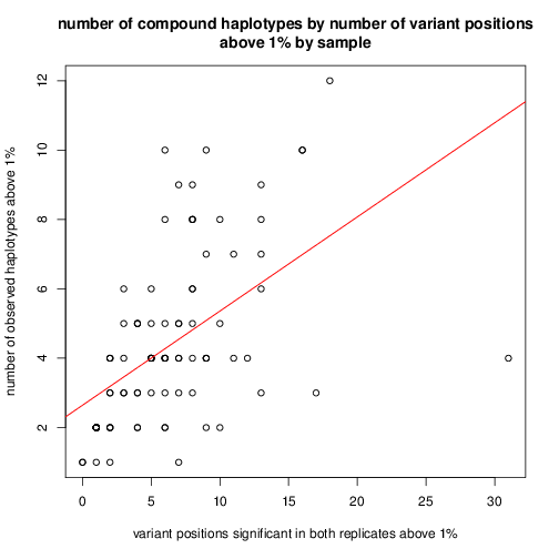
look at number of variant positions observed versus number of
compounds > 1%
Look at whether the number of compounds greater than 1% is related to
the number of variant positions with abundance greater than 1%:
summary(mylm)
Coefficients:
Estimate Std. Error t value Pr(>|t|)
(Intercept) 2.64463 0.36252 7.295 1.13e-10 ***
mm[, 2] 0.27142 0.04557 5.956 4.92e-08 ***
---
Signif. codes: 0 ‘***’ 0.001 ‘**’ 0.01 ‘*’ 0.05 ‘.’ 0.1 ‘ ’ 1
Residual standard error: 2.115 on 90 degrees of freedom
Multiple R-squared: 0.2828, Adjusted R-squared: 0.2748
F-statistic: 35.48 on 1 and 90 DF, p-value: 4.917e-08
The number of compounds greater than 1% is about 27% of the number of
variant positions above 1%.
 ================================
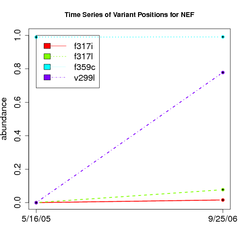
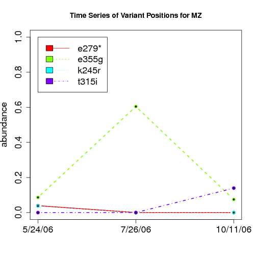
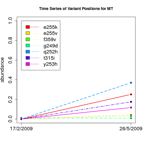
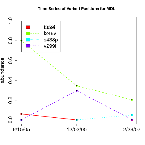
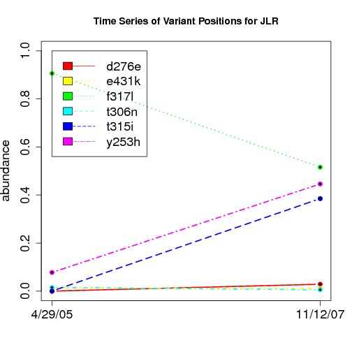
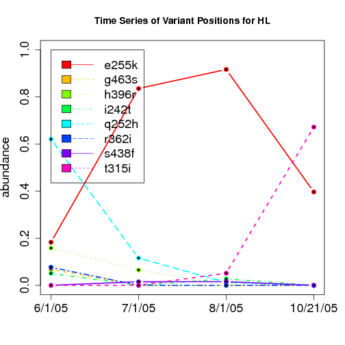
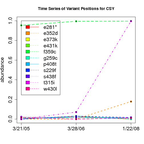
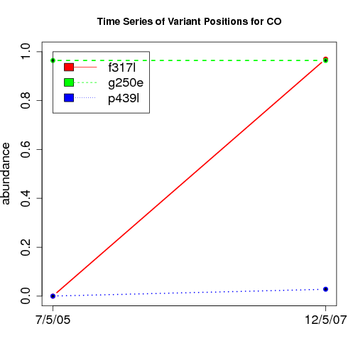
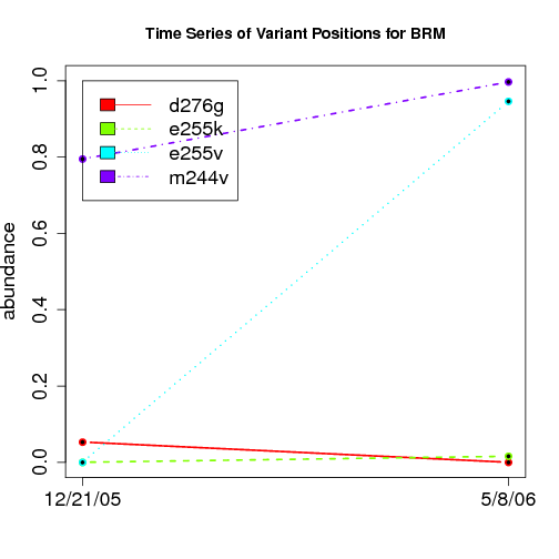
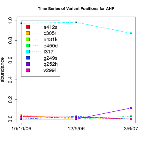
time evolution
For the patients with multiple time points, show the time evolution.
here are the patients with more than 1 timepoint:
30 HL 4
4 AHP 3
14 CSY 3
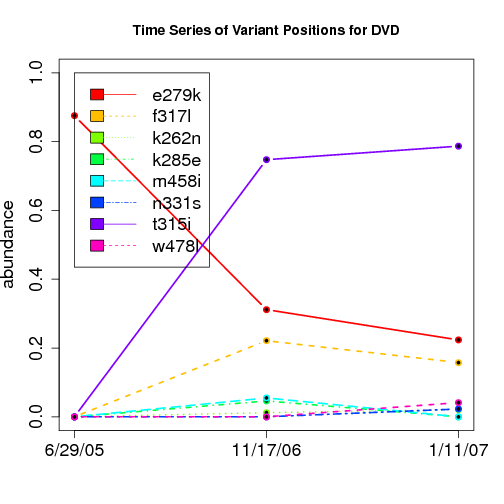
22 DVD 3
52 MDL 3
56 MZ 3
7 BRM 2
10 CO 2
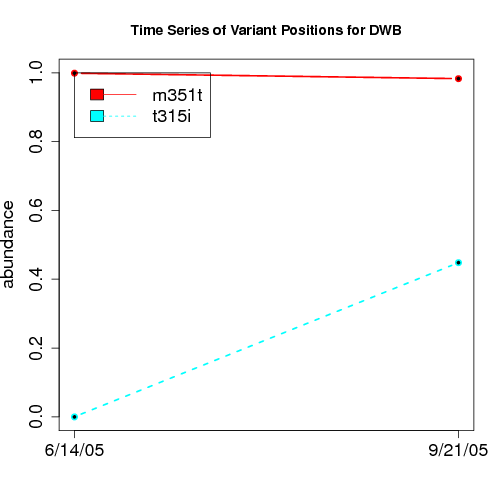
23 DWB 2
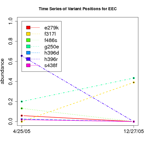
26 EEC 2
37 JLR 2
55 MT 2
57 NEF 2
Here are the time series plots for all variants where the mean
aboundace is greater than 0.0075. PatientID in filename.
 ================================
Compound Variants
I looked for interesting patterns in compound variants for those
patients with time series.
-- EEC has two codons for same variant f317l (tta,ctc) at the second time point:
key count fraction variant limsID barcode.x
10167 2450177-0036.F2 27 0.021669 g250e.gag,f317l.ctc 2450177-0036 F2
10168 2450177-0036.F2 62 0.049759 g250e.gag,f317l.tta 2450177-0036 F2
10169 2450177-0036.F2 131 0.105136 f317l.ctc 2450177-0036 F2
10170 2450177-0036.F2 204 0.163724 g250e.gag 2450177-0036 F2
10171 2450177-0036.F2 251 0.201445 f317l.tta 2450177-0036 F2
10172 2450177-0036.F2 507 0.406902 2450177-0036 F2
-- CSY is heavily compounded
21/3/05: f359c
 28/3/06: f359c and low level t315i+f359c
 22/1/08: t315i+f359c and 4 variant compound at >5%
 tmp=compvars[compvars$ptInit=="CSY" & compvars$fraction>0.01,]; split(tmp,tmp$key,drop=T)
$`2450177-0032.F1`
key count fraction variant limsID barcode.x
6391 2450177-0032.F1 26 0.010874 p230p.cca,f359c.tgc 2450177-0032 F1
6392 2450177-0032.F1 606 0.253450 2450177-0032 F1
6393 2450177-0032.F1 1325 0.554161 f359c.tgc 2450177-0032 F1
$`2450177-0032.F2`
key count fraction variant limsID barcode.x
6818 2450177-0032.F2 58 0.023529 t315i.att,f359c.tgc 2450177-0032 F2
6819 2450177-0032.F2 334 0.135497 2450177-0032 F2
6820 2450177-0032.F2 1006 0.408114 f359c.tgc 2450177-0032 F2
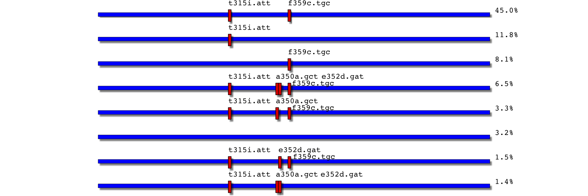
$`2450177-0032.F3`
key count fraction variant
6985 2450177-0032.F3 21 0.010479 t315i.att,a350a.gct,e352d.gat
6986 2450177-0032.F3 21 0.010479 t315i.att,a350a.gct
6987 2450177-0032.F3 36 0.017964 t315i.att,e352d.gat,f359c.tgc
6988 2450177-0032.F3 65 0.032435
6989 2450177-0032.F3 78 0.038922 t315i.att,a350a.gct,f359c.tgc
6990 2450177-0032.F3 118 0.058882 t315i.att,a350a.gct,e352d.gat,f359c.tgc
6991 2450177-0032.F3 140 0.069860 f359c.tgc
6992 2450177-0032.F3 244 0.121756 t315i.att
6993 2450177-0032.F3 903 0.450599 t315i.att,f359c.tgc
================================
tmp=compvars[compvars$ptInit=="CSY" & compvars$fraction>0.01,]; split(tmp,tmp$key,drop=T)
$`2450177-0032.F1`
key count fraction variant limsID barcode.x
6391 2450177-0032.F1 26 0.010874 p230p.cca,f359c.tgc 2450177-0032 F1
6392 2450177-0032.F1 606 0.253450 2450177-0032 F1
6393 2450177-0032.F1 1325 0.554161 f359c.tgc 2450177-0032 F1
$`2450177-0032.F2`
key count fraction variant limsID barcode.x
6818 2450177-0032.F2 58 0.023529 t315i.att,f359c.tgc 2450177-0032 F2
6819 2450177-0032.F2 334 0.135497 2450177-0032 F2
6820 2450177-0032.F2 1006 0.408114 f359c.tgc 2450177-0032 F2
$`2450177-0032.F3`
key count fraction variant
6985 2450177-0032.F3 21 0.010479 t315i.att,a350a.gct,e352d.gat
6986 2450177-0032.F3 21 0.010479 t315i.att,a350a.gct
6987 2450177-0032.F3 36 0.017964 t315i.att,e352d.gat,f359c.tgc
6988 2450177-0032.F3 65 0.032435
6989 2450177-0032.F3 78 0.038922 t315i.att,a350a.gct,f359c.tgc
6990 2450177-0032.F3 118 0.058882 t315i.att,a350a.gct,e352d.gat,f359c.tgc
6991 2450177-0032.F3 140 0.069860 f359c.tgc
6992 2450177-0032.F3 244 0.121756 t315i.att
6993 2450177-0032.F3 903 0.450599 t315i.att,f359c.tgc
================================